Frontiers

The geochemical composition of glauconitic clasts is a provenance marker to distinguish the origin of gravity flows in sedimentary basins. Their geochemical variation is visible in major and trace elements composition, where the former can be visualized by element mapping of glauconitic clasts. By applying automated quantitative mineralogy on a Scanning Electron Microscope equipped with the ZEISS Mineralogic™ software platform, we developed a new way to visualize the element distribution in selected minerals, while masking out the other minerals simultaneously. This software applies energy dispersive spectroscopy spectrum deconvolution for each analysis point, therefore quantitative concentrations (wt%) of each element are determined for each pixel and visualized in the false-coloured element map with reproducible results for individual grains and zonations in these grains. The investigated glauconitic clasts were collected from eleven drill cores, covering a 1400 m-depth interval, and crosscutting four different gravity flow members. The clasts show three different trends: first, cores of glauconitic clasts show a variation of compositions that are mainly dependent on the conditions during their formation. This is most visible for Si and Al. Secondly, the composition of the glauconitic clasts changes with depth, their cores become first more, than less Fe-rich and more K-rich. This is probably an alteration effect, depending on temperature, and therefore mineral stability. And, thirdly, most glauconitic clasts are zoned, where rims are richer in Al and poorer in Fe and K. The visualization of the chemical variation in the glauconitic clasts proofs to be a useful tool to separate these conflicting element exchange processes.

The Scanning Electron Microscope (SEM) can be applied in different ways to perform an element mapping of the sample to visualize the distribution of individual elements across the sample. Traditional element mapping is performed with the software provided together with the energy dispersive spectroscopy (EDS) detector on the SEM, where an energy window in the analysed spectrum is selected in the software and screened for X-rays with the relevant energy. Results are typically provided as relative intensities, compared to high values within the sample. This makes it hard to compare between samples, especially if they do not both have the same composition. A second disadvantage of this technique is that several elements may have peaks in the same energy window. The rise of automated quantitative mineralogy (AQM) analysis techniques allowed for element mapping by the matching of spectra against a database (e.g., Gottlieb et al., 2000; Gäbler et al., 2011). There, reference spectra with small variations in composition could be included in the databases, which omitted the problem of peak overlap created by the energy windows. However, there will still be an uncertainty in the precise concentrations of the minor elements in the spectrum. Here, we applied the ZEISS Mineralogic software platform for the AQM, which applies a full spectrum deconvolution for every analytical point by applying the single spectrum mode of the EDS software. Therefore, semi-quantitative results are available in weight (wt)% concentrations for every pixel in the generated mineral map. This presents a hitherto unused potential for precise element mapping on single minerals in a mixed aggregate.

Samples in this study are derived from cores into partially depleted oil fields in Siri Canyon in the Danish North Sea, which are currently under consideration as sites for CO2 storage. The oil fields are in glauconitic sandstones, a reservoir type, which has not previously been tested for CO2 storage. Since glauconitic clasts comprise 20–30 vol% of the sandstones (Weibel et al., 2010; Kazerouni et al., 2012), they may potentially have large influence on the CO2 reservoir stability. Glauconitic clasts occur with substantial variations, both in coloration, morphologically, structurally, and chemically (e.g., Odin and Matter 1981; Amorosi 1997; Kelley and Webb 1999; Meunier and El Albani 2007; Rudmin et al., 2017). Therefore, the AQM analysis has been applied to map compositional variations.

Glauconite is an iron (Fe)-rich, potassium (K)-poor mica that can be interstratified with minerals of the smectite-group. Glauconitic clasts form by glauconitisation of different particles in the shallow marine environment, upper slope and the outer shelf (50–500 m water depth; e.g., Odin and Matter 1981; Van Houten and Purucker 1984; Kelley and Webb 1999; Meunier and El Albani 2007; Rudmin et al., 2017). Various parent minerals have been identified, such as degraded micaceous clay minerals, carbonate clasts, argillaceous/fecal pellets, bioclasts, feldspar, rock fragments (e.g., Odin and Matter 1981; Sánchez-Navas et al., 2008; Banerjee et al., 2016; Tribovillard et al., 2021; Tounekti et al., 2021). Glauconitic clasts are known for their greenish colour and formed as pellets or by weathering of biotite or other 2:1-stratified micaeous minerals in shallow marine environment, near a coast with relatively warm water and at reducing conditions (McRae 1972). Compositional differences correlate with the different ratios of illite and smectite layers in the glauconitic clasts, which can be determined by X-ray diffraction techniques as an average for all glauconitic clasts in the sample (McRae 1972). However, individual glauconitic clasts can show considerable variation within a single sample and individual glauconitic clasts may show a different composition in the rim and the core of the clast (Velde and Odin 1975).

Elemental variations in glauconitic clasts are used in provenance and to explain processes active in the shallow marine environment during their formation (e.g., Meunier and El Albani 2007; Baldermann et al., 2017) but also in diagenetic studies to explain changes in composition with depth (e.g. Kazerouni et al., 2012; Bansal et al., 2017). Both the formation processes and the diagenetic alterations include the same set of elements, which might be problematic for the interpretation of the glauconitic bulk chemical data. Hence, the aim of this contribution is two-fold: Firstly, we present a new method for mineral-specific element mapping. Secondly, we apply this new method in a case study on glauconitic clasts, where we try to resolve different processes acting on these clasts by element mapping with the aim to differentiate between provenance and formation-related processes versus diagenetic changes.

AQM of glauconitic sandstones were performed on the SEM at the Geological Survey of Denmark and Greenland (GEUS), using the ZEISS Mineralogic software platform. Analyses were performed with acceleration voltages of 12–15 kV, a 120 μm2 aperture. Analysis time per spectrum is set such that each spectrum contains at least 2,500 counts. For AQM, the backscattered electron contrast (BSE) is applied to display the contrast between different mineral phases in the sample. During AQM, a mosaic of BSE frames of a representative part of the sample is compiled. Each frame in the mosaic is thereafter analysed with the EDS detectors applying a user-defined step-size of 0.5–20 µm between EDS analytical spots. The chemistry in each spot is interpreted as a mineral species, which is forming one pixel in the false-coloured mineral map. Oxygen is quantified as one of the elements in the spectrum and resulting quantities are normalized to 100%. The classification of minerals is operator-based, where obtained mineral compositions are compared to known compositions in Deer et al. (1985) and the online database www.webminerals.com. Further details on the software and applied method can be found in Keulen et al. (2020). The precision of the analyses in this study were tested by repeating analyses on the same samples, where the concentration of the major elements could be reproduced within 1 wt%.

Most thin sections have been investigated several times at different magnifications and step-sizes to obtain both an overview over the bulk mineralogy, grain size distribution and the range of glauconitic compositions at low magnifications, and on the internal structure of glauconitic clasts at higher magnifications applying smaller step sizes. For the high-magnification maps created with a step-size of 0.5 µm, analyses were performed at 12 kV, to ensure a small interaction volume for the incoming electron beam with the analysed thin section and to avoid a mixed EDS signal from neighbouring clasts. Graham and Keulen (2019) showed that circa 50% of the EDS signal comes from an area less than 250 nm in diameter when applying 10 kV. By applying the same technique, we can show that for glauconitic clasts analysed at 12 kV, 80% of the EDS signal comes from a 0.5 µm-wide interaction volume (see Supplementary Figure S1).

The Mineralogic software has been applied to create element maps of the samples for individual minerals in the sample, while the other minerals are blanked. This is possible, because the mineral maps created with ZEISS Mineralogic are based on EDS spectrum deconvolution for every single pixel, including matrix quantification (Phi-Rho-Z or ZAF), omission of escape peaks and double peaks, like for a single spot EDS measurement. Therefore, quantitatively determined element wt% concentrations are available for each pixel in the mineral map (see also Keulen et al., 2020 for further description; Figure 1). A new mineral list was created for the false-colour mineral map, in which all minerals, except for the mineral of interest, are now coloured white, and the target mineral is coloured by concentrations of specific elements in the mineral, e.g., the Fe concentration in glauconite (see Figures 2 and Supplementary Figure S2, Figure 3). In this way, mineral-specific element maps can be created, with absolute element concentrations, and these concentrations can be used to draw diagrams (Figure 4).

F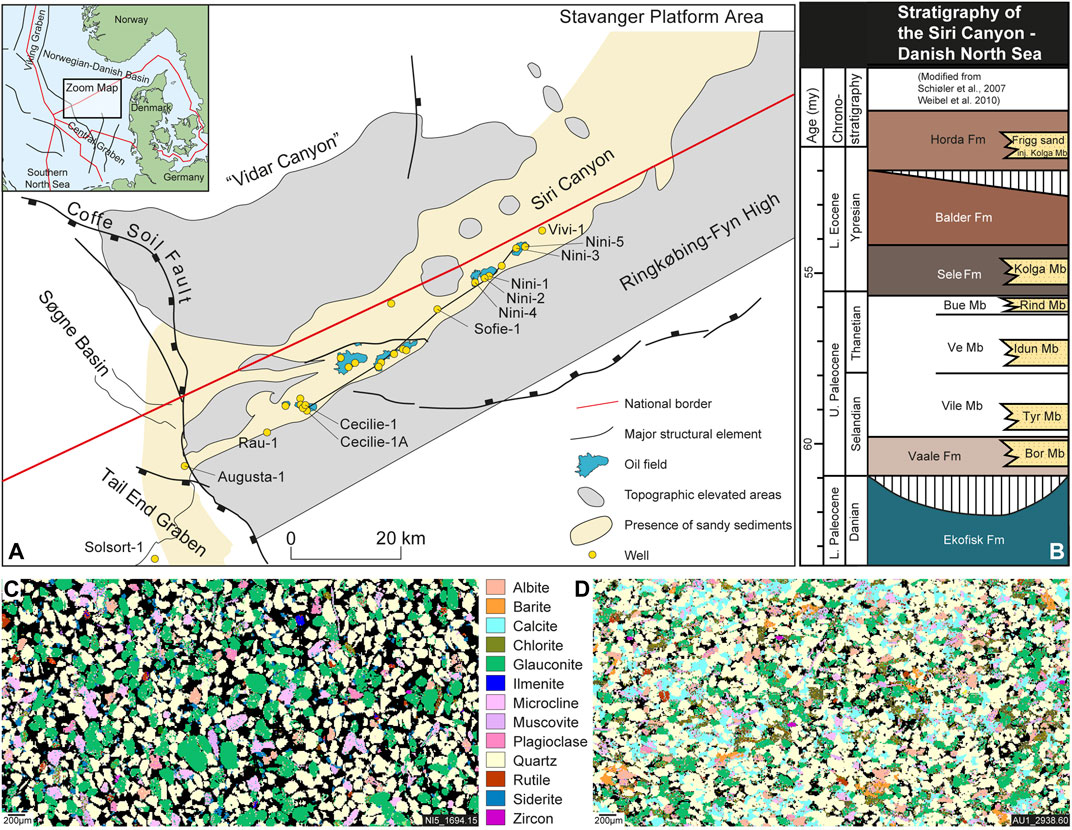IGURE 1. (A) Map showing wells and oil fields in the Siri Canyon area, modified after Friis et al. (2007). Wells indicated by name has been applied in the study. (B) Stratigraphy of the Siri Canyon. (C) AQM mineral map of the shallowest sample. (D) AQM mineral map of one of the deepest buried sample.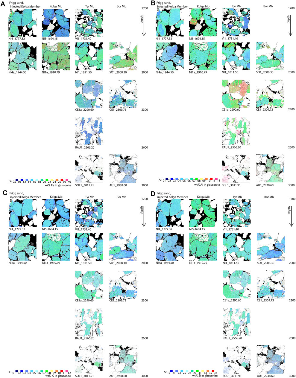

FIGURE 2. Variation in glauconitic clast composition of the five studied sand-flows for the elements (A) iron (Fe), (B) aluminium (Al), (C) potassium (K) and (D) silicon (Si) with increasing depth. All other minerals in the sample are coloured white. Porosity in the sample is shown in black. A large version of the figure is provided as Supplementary Figure S2.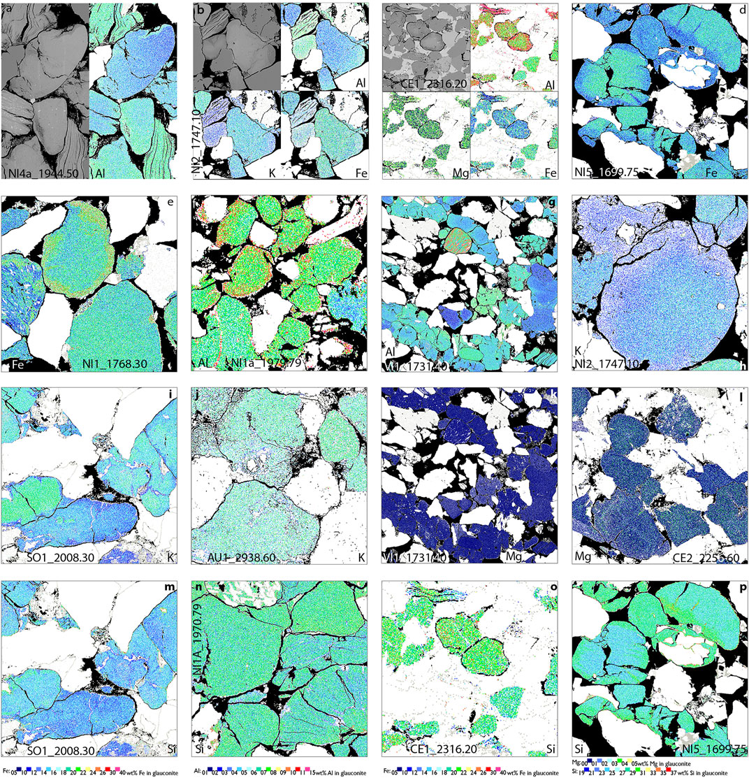

FIGURE 3. Details of glauconitic clasts’ cores, rims and fractures from the Siri Canyon. See text for details. Grey-scale images are BSE micrographs.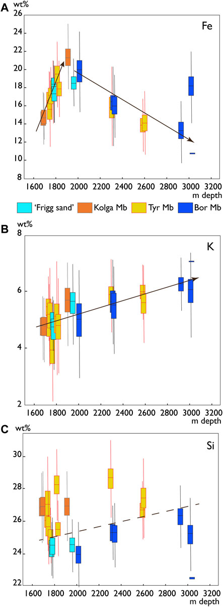

FIGURE 4. Glauconitic clast chemistry per sample from different gravity flows plotted per member after their sampling depth. (A) Fe, (B) K, and (C) Si. Dashed line visualizes separation between members with low and high Si concentration.

We have applied this technique on a set of 22 thin sections of glauconitic sands from the Siri Canyon in the Danish North Sea Basin (see Figure 1). Siri Canyon is characterized by Palaeocene hemipelagic mudstone and marls, intercalated with glauconitic sand deposited by mass flow and turbidites (Hamberg et al., 2005; Schiøler et al., 2007). Remobilisation of the sand after deposition resulted in injectites in both stratigraphically younger and older strata (Svendsen et al., 2010). The samples were collected from 13 cored wells with varying present-day burial depths of 1,694–3019 m depth and represent four different gravity flows, Bor, Tyr, Kolga members and Frigg sand (Figure 1). Note, that Frigg sand is an informal denotation of presumably Kolga Member, which is injected into a stratigraphically higher level, i.e., the Horda Formation. Samples were collected from the center of the glauconitic sand intervals. Only a few gravity flows were present in each well. The glauconitic sands are homogeneous in composition, with circa 50% quartz, around 20–30% glauconitic minerals in the shallow part of the Siri Canyon (Weibel et al., 2010). The remaining minerals are 10% feldspars, 0–7% carbonates (mainly siderite) and very minor muscovite, biotite, other clays, metamorphic minerals, accessory minerals, rock salt and pyrite. The samples are remarkably homogeneous in composition and grain size (see also Hamberg et al., 2005; Friis et al., 2007). The gravity flows originate from the Stavanger platform and are deposited as dipping members. The individual drill cores reached the same members at different burial depths, thus the effect of provenance versus alteration at higher depth/temperature could be investigated within the glauconitic gravity flows.

The variation in glauconitic clast composition has been studied from element maps for iron (Fe), aluminium (Al), magnesium (Mg), potassium (K), and silicon (Si). In Figures 2; Supplementary Figure S2 the element maps have been sorted by the individual members of the Siri Canyon. Most glauconitic clasts, irrespective of their member, drill core or depth have a core and a rim. Many have internal fractures along which a change in element composition has been observed. In most samples, the glauconitic clasts nearly all have a similar composition, within a few wt% margin. However, some samples, especially those at shallow depth, show a very wide range of compositions, for example Vi1_1731.40 (uppermost Tyr Member) in Figures 2; Supplementary Figure S2. Glauconitic grains that still show a mica-cleavage usually are more Al-rich and more depleted in Fe-K than surrounding glauconitic clasts (see e.g. Figures 3A,B and Supplementary Figure S2).

Here, we shortly discuss some trends of the element distribution with depth, between different members and between drill cores.

The Fe in the crystal structure of glauconitic minerals can be replaced by aluminium (Fe3+/Al3+ exchange) and by magnesium (Fe2+/Mg2+ exchange). The concentration of Fe strongly anticorrelates with aluminium, and much less with Mg (Figure 3C, Supplementary Figure S2). As a rule of thumb, glauconite has typically twice as much Mg as Fe2+ (Odom 1984). As Mg concentrations are low in the samples, Fe2+ will be low too, and therefore, a strong anticorrelation of Fe with Al is expectable as most present Fe will be of the Fe3+ variety.

As a general trend, samples collected at approximately 1900–2000 m depth have the highest Fe concentrations. Fe-concentrations decreases with depth and are also low around 1700 m-depth (Figure 4A). This is especially notable in the uppermost Kolga Member sample (Ni5_1,694.15) which is significantly poorer in Fe than the deeper samples (Figures 2; Supplementary Figure S2). There is no clear trend for Fe per member or per drill core, thus variation in Fe concentrations does not seem to be a lateral variation. In nearly all samples, lower Fe-concentrations are recorded around fractures and at the rims of the clasts. This, too, is opposed to Al behaviour (and not seen in Mg) thus an Fe-Al exchange reaction (Figures 3C, D). In few clasts, for example the one in Ni1-1768.30 (Figure 3E) a more Fe-rich rim than core is observed. This is most likely caused by a reaction with an iron-rich parent mineral.

The amount of Al in glauconitic clasts does not change significantly with depth for the shallower samples (shallower than 2000 m), but the concentration increases with depth for samples from the deeper parts of the Siri Canyon (Figures 2; Supplementary Figure S2). Variations in the Al composition seem to vary more between members in the Siri Canyon (compare Figure 3A (Frigg sand) to Figure 3F (Kolga Member), both from the same depth) and also between clasts from the same sample (Figures 2; Supplementary Figure S2 and Figure 3G). As described above for Fe, there is a strong anti-correlation between Fe and Al and this is clearly reflected in the more Al-rich rims around the glauconitic clasts and more Al in fractures in the clasts (Figures 3B, C, F, G).

The concentration of K in glauconitic clasts increases with depth (Figures 3H–J; Figure 4B). There are no clear trends visible for individual members (Figures 2, Supplementary Figure S2). Nevertheless, the amount of K decreases from the core of the clasts towards the rims, within the same glauconitic clast (Figures 3H, I). Around fractures, glauconitic clasts are poorer in K than the surrounding material (Figure 3I).

The amount of Mg in glauconitic clasts is low in nearly all samples. Even though Mg can range between 1 and 5 wt%, the majority of samples has Mg concentrations of 0–2 wt% (see Figures 3K, L; Supplementary Figure S2; with the notable exception of Figure 3C). Like for Fe, there is neither a clear correlation with depth of the samples, nor a differentiation between members for Mg (Supplementary Figure S2). Also, only very minor variation within a single sample exists (Figure 3K, compare to Figure 3G, Al). Most samples do not show a clear core-rim structure. Some samples seem to have higher Mg concentrations near cracks (Figure 3L), but this trend is not as clear as for Fe, K and Al.

Silicon in glauconitic clasts shows a very weak correlation with depth. However, Si shows a clear trend per member of the Siri Canyon (Figures 2; Supplementary Figure S2). The Tyr and Kolga Members are more Si-rich than the other two members (compare Figure 3M (Bor Member) to Figure 3N (Kolga Member), Figure 4C). Note, that the “Frigg sand”, injected Kolga Member according to Svendsen et al. (2010), show clear differences to Kolga Member (Figure 2). There are only few glauconitic clasts with a clear core-rim structure or alterations along fractures (compare Figure 3C with Figure 3O, where the core-rim structure is not visible; and Figure 3D with Figure 3P where these are remained). Some clasts also show a patchy internal structure with broad rims (e.g., Figure 3M, compare to Figure 3I (K)).

Different processes seem to play a role in the element exchange in glauconitic clasts and each of the studied elements show their own pattern. Three different processes affect the compositions: 1) variations with depth, 2) core versus rim differences and 3) provenance variations. These will be discussed separately.

Aluminium and especially silicon vary between the cores of glauconitic clasts from members in the Siri Canyon collected at the same depth. This trend is mildly visible for the plot with Fe, although not in K and Al (Figure 2; Supplementary Figure S2). Glauconites derived from specific parent rocks generally have different maturity and carry unique geochemical and mineralogical properties. A difference in provenance is ultimately a difference in the glauconitisation process on the outer shelf (Amorosi 1997). During glauconitisation and early diagenesis, K, and afterwards Fe are built into the crystal lattice and replace Al and Si (Odom 1984; Amorosi 1997; Bansal et al., 2017). Harder 1980 showed with experiments that the Si-concentration of the pore water is the determining factor in the formation of glauconite, while high K-concentrations are also important. Different concentrations in the pore water may affect the Si-concentrations in the glauconitic cores. The provenance characteristics of the samples is therefore both determined by the mineralogy of their precursor particles and by chemical processes during glauconitisation. This is visible in Figure 4C, where the “Frigg sand” and Bor Member consequently have lower Si concentrations than Kolga and Tyr Members.

Further diagenesis is visible as increase of Fe with depth (here down to circa 2000 m, Figure 2; Supplementary Figure S2) and the increase in K in the samples (conform with observations by e.g., Bansal et al., 2017). This fits well with observations from Strickler and Ferrell (1990), who describe that Fe3+ incorporation in glauconite occurs between 600 and 1800 m depth. Meunier and El Albani (2007) describe that this is a time and sedimentation/cementation rate-depending process. This diagenetic process is visible in the cores of the glauconitic clasts (Figures 2; Supplementary Figure S2).

Deeper than 2000 m, Fe might decrease again because a different clay mineral in the glauconitic clasts becomes more stable, e.g., illite instead of smectite, allowing for less Fe, but increasing amounts of K and Al in the clasts. Kazerouni et al. (2012) indicate for samples from the same canyon system that around 2000 m depth a change in the mineralogic structure of glauconitic clasts occurs. Deeper than 2000 m, the mixed-layer illite/smectite is well ordered and slightly more illite-rich. They observe a decrease in Fe-concentration, as well as an increase in Si. The latter cannot be confirmed in the current study, but this might be explained by comparing different members with different Si-concentrations (Figures 2; Supplementary Figure S2 and Figure 4), or by the presence of micrometre-sized quartz grains in the glauconitic clasts (here excluded from the analysis).

Figure 3 shows that Al is enhanced in the rims compared to cores, while Fe and K concentrations are clearly lower in rims and cracks; Mg does not show clear variations from core to rim, and Si only shows changes in concentrations irregularly. Bansal et al. (2017) give two explanations for the rims in glauconitic clasts related to late diagenetic alteration: they are either an intermediate stage in reaction of glauconitic smectite to glauconitic mica (Velde and Odin 1975; Odom 1984) or a result of interaction with meteoric water or brine. As the investigated glauconitic sandstones were not involved in uplift in the later part of their history, the first explanation is more likely. Due to this alteration, K and Fe decrease, while Al and Si increase. The sharp contrast between the core and the rim suggests that this alteration is not a continuous process at depth, but one that starts suddenly after a change in the ambient conditions (e.g., temperature, fluid composition).

Most observed glauconitic element distributions fit well with previously described processes in glauconitic clasts’ formation and alteration. The novelty of this contribution lies in the ability to visualise these changes with mineral-specific quantitative element mapping. Our mapping shows that the Si-concentration in glauconitic clasts can vary strongly between gravity flows, which was not demonstrated in this way before. The Si concentration is determined early in the glauconisation process and is thus a provenance marker. We show considerable differences between the Kolga Member and the injected Kolga Member, suggesting that possibly not all “Frigg sand” is injected Kolga Member. The detailed element mapping show that the element concentrations within individual glauconitic clasts and between neighbouring clasts may vary considerably. Therefore, analytical methods that take average glauconitic concentrations might therefore not consider the effect of late-stage diagenetic alteration effects.

Due to this newly developed element mapping technique with complete spectrum deconvolution, mineral maps could be created for individual minerals in the samples, while the software masked out the other minerals based on their chemistry. Thus, inclusions (e.g., quartz, apatite), alteration minerals (e.g., berthierine or chlorite), or precursor minerals (e.g., biotite) were not included in the element maps. Therefore, only the parts with a glauconitic compositions were element mapped, even where the different minerals are closely intermixed. For example, in sample Ni2_1747.10 (Figure 3H) the rim of the glauconitic clast is less dense in colour than the core, due to partial replacement by authigenic phases (white). To our knowledge, this is the first time that such mineral-specific quantitative element mapping was applied, and the advantages are large and widely applicable both within and outside Earth Sciences.

Because the element concentrations are semi-quantitatively determined absolute values wt% and recorded for every analysed pixel in the false-coloured mineral map, these absolute concentrations can be extracted and applied in graphs that describe the development of the samples’ chemistry with depth and time. Geochemical data for the glauconitic clasts can be extracted from the mineral maps, excluding all other phases. Figure 4 shows that the glauconitic clasts not only can be visualized by mineral-specific element mapping, but also that their data can be used in quantitative studies. Hence, this technique is both a quantitative tool and a novel way of visualizing geochemical data.

The raw data supporting the conclusions of this article will be made available by the authors, without undue reservation.

NK wrote the manuscript, developed the mineral-specific quantitative element mapping and made the figures. RW managed the greensand petrography project, wrote part of the text and provided data for Supplementary Table S1. SNM conducted most analyses. All authors reviewed the final manuscript.

This study was funded by the Danish Energy Technology Development and Demonstration Program (EUDP) and accomplished by a consortium consisting of GEUS, INEOS, Maersk Drilling and Wintershall DEA. GEUS contributed to publishing the data.

The authors declare that the research was conducted in the absence of any commercial or financial relationships that could be construed as a potential conflict of interest.

All claims expressed in this article are solely those of the authors and do not necessarily represent those of their affiliated organizations, or those of the publisher, the editors and the reviewers. Any product that may be evaluated in this article, or claim that may be made by its manufacturer, is not guaranteed or endorsed by the publisher.

We cordially thank Henrik Friis for sharing his knowledge on the Siri Canyon greensands and for the loan of part of the thin sections. reviewers with constructive comments are thanked for their help to improve this publication. This paper is published with the acceptance of GEUS.

The Supplementary Material for this article can be found online at: https://www.frontiersin.org/articles/10.3389/feart.2022.788781/full#supplementary-material

Amorosi, A. (1997). Detecting Compositional, Spatial, and Temporal Attributes of Glaucony: a Tool for Provenance Research. Sediment. Geol. 109, 135–153. doi:10.1016/s0037-0738(96)00042-5

CrossRef Full Text | Google Scholar

Baldermann, A., Dietzel, M., Mavromatis, V., Mittermayr, F., Warr, L. N., and Wemmer, K. (2017). The Role of Fe on the Formation and Diagenesis of Interstratified Glauconite-Smectite and Illite-Smectite: A Case Study of Upper Cretaceous Shallow-Water Carbonates. Chem. Geol. 453, 21–34. doi:10.1016/j.chemgeo.2017.02.008

CrossRef Full Text | Google Scholar

Banerjee, S., Bansal, U., and Thorat, A. V. (2016). A review on Palaeogeographic Implications and Temporal Variation in Glaucony Composition. Sediment. Geol., 43–71.

CrossRef Full Text | Google Scholar

Bansal, U., Banerjee, S., Pande, K., Arora, A., and Meena, S. S. (2017). The Distinctive Compositional Evolution of Glauconite in the Cretaceous Ukra Hill Member (Kutch Basin, India) and its Implications. Mar. Petroleum Geol. 82, 97–117. doi:10.1016/j.marpetgeo.2017.01.017

CrossRef Full Text | Google Scholar

Deer, W. A., Howie, R. A., and Zussmann, J. (1985). An Introduction to Rock-Forming Minerals. Essex: Longman Group Limited, 528.

Google Scholar

Friis, H., Poulsen, M. L. K., Svendsen, J. B., and Hamberg, L. (2007). Discrimination of Density Flow Deposits Using Elemental Geochemistry-Implications for Subtle Provenance Differentiation in a Narrow Submarine Canyon, Palaeogene, Danish North Sea. Mar. Petroleum Geol. 24, 221–235. doi:10.1016/j.marpetgeo.2007.02.001

CrossRef Full Text | Google Scholar

Gäbler, H.-E., Melcher, F., Graupner, T., Bahr, A., Sitnikova, M. A., Henjes-Kunst, F., et al. (2011). Speeding up the Analytical Workflow for Coltan Fingerprinting by an Integrated Mineral Liberation Analysis/LA-ICP-MS Approach. Geostand. Geoanal. Res. 35, 431–448. doi:10.1111/j.1751-908X.2011.00110.x

CrossRef Full Text | Google Scholar

Gottlieb, P., Wilkie, G., Sutherland, D., Ho-Tun, E., Suthers, S., Perera, K., et al. (2000). Using Quantitative Electron Microscopy for Process Mineralogy Applications. JOM 52, 24–25. doi:10.1007/s11837-000-0126-9

CrossRef Full Text | Google Scholar

Graham, S., and Keulen, N. (2019). Nanoscale Automated Quantitative Mineralogy: A 200-nm Quantitative Mineralogy Assessment of Fault Gouge Using Mineralogic. Minerals 9, 665. doi:10.3390/min9110665

CrossRef Full Text | Google Scholar

Hamberg, L., Dam, G., Wilhelmson, C., and Ottesen, T. G. (2005). “Paleocene Deep-Marine Sandstone Plays in the Siri Canyon Offshore Denmark, Southern NorwaySynthesis of Glauconite at Surface Temperatures,” in Petroleum Geology: North-West Europe and Global Perspectives. Editors A.G Dore, and B. A Vining (London: Geological Society), 28, 1185217–1198222. Proceedings of the 6th Petroleum Geology Conference. doi:10.1144/0061185

CrossRef Full Text | Google Scholar

Harder, H. (1980). Syntheses of Glauconite at Surface Temperatures. Clays and Clay Minerals 28 (3), 217–222. doi:10.1346/ccmn.1980.0280308

CrossRef Full Text | Google Scholar

Kazerouni, A. M., Poulsen, M. L. K., Friis, H., Svendsen, J. B., and Hansen, J. P. V. (2012). Illite/smectite Transformation in Detrital Glaucony during Burial Diagenesis of Sandstone: A Study from Siri Canyon - Danish North Sea. Sedimentology 60, 679–692. doi:10.1111/j.1365-3091.2012.01356.x

CrossRef Full Text | Google Scholar

Kelley, J. C., and Webb, J. A. (1999). The Genesis of Glaucony in the Oligo–Miocene Torquay Group, Southeastern Australia: Petrographic and Geochemical Evidence. Sediment. Geol. 125, 99–114. doi:10.1016/S0037-0738(98)00149-3

CrossRef Full Text | Google Scholar

Keulen, N., Malkki, S. N., and Graham, S. (2020). Automated Quantitative Mineralogy Applied to Metamorphic Rocks. Minerals 10 (1), 47. doi:10.3390/min10010047

CrossRef Full Text | Google Scholar

McRae, S. G. (1972). Glauconite. Earth-Science Rev. 8, 397–440. doi:10.1016/0012-8252(72)90063-3

CrossRef Full Text | Google Scholar

Meunier, A., and El Albani, A. (2007). The glauconite?Fe-illite?Fe-Smectite Problem: a Critical Review. Terra nova. 19, 95–104. doi:10.1111/j.1365-3121.2006.00719.x

CrossRef Full Text | Google Scholar

Odin, G. S., and Matter, A. (1981). De Glauconiarum Origine. Sedimentology 28, 611–641. doi:10.1111/j.1365-3091.1981.tb01925.x

CrossRef Full Text | Google Scholar

Odom, I. E. (1984). 13. GLAUCONITE and CELADONITE MINERALS. Rev. Mineralogy Geochem. 13 (1), 545–572. doi:10.1515/9781501508820-017

CrossRef Full Text | Google Scholar

Rudmin, M., Banerjee, S., and Mazurov, A. (2017). Compositional Variation of Glauconites in Upper Cretaceous-Paleogene Sedimentary Iron-Ore Deposits in South-Eastern Western Siberia. Sediment. Geol. 355, 20–30. doi:10.1016/j.sedgeo.2017.04.006

CrossRef Full Text | Google Scholar

Sánchez-Navas, A., Martín-Algarra, A., Eder, V., Reddy, B. J., Nieto, F., and Zanin, Y. N. (2008). Color, Mineralogy and Composition of Upper Jurassic West Siberian Glauconite: Useful Indicators of Paleoenvironment. Can. Mineralogist 46, 1249–1268. doi:10.3749/canmin.46.5.1249

CrossRef Full Text | Google Scholar

Schiøler, P., Andsbjerg, J., Clausen, O. R., Dam, G., Dybkjær, K., Hamberg, L., et al. (2007). Lithostratigraphy of the Palaeogene – Lower Neogene Succession of the Danish North Sea. Geol. Surv. Den. Greenl. Bull. 12, 77.

Google Scholar

Strickler, M. E., and Ferrell, R. E. (1990). Fe Substitution for Al in Glauconite with Increasing Diagenesis in the First Wilcox Sandstone (Lower Eocene), Livingston Parish, Louisiana. Clays Clay Minerals 38, 69–76. doi:10.1346/ccmn.1990.0380110

CrossRef Full Text | Google Scholar

Svendsen, J. B., Hansen, H. J., Staermose, T., and Engkilde, M. K. (2010). Sand Remobilization and Injection above an Active Salt Diapir: the Tyr Sand of the Nini Field, Eastern North Sea. Basin Res. 22, 548–561. doi:10.1111/j.1365-2117.2010.00480.x

CrossRef Full Text | Google Scholar

Tounekti, A., Boukhalfa, K., Choudhury, T. R., Soussi, M., and Banerjee, S. (2021). Global and Local Factors behind the Authigenesis of Fe-Silicates (Glauconite/Chamosite) in Miocene Strata of Northern Tunisia. J. Afr. Earth Sci. 184, 104342. doi:10.1016/j.jafrearsci.2021.104342

CrossRef Full Text | Google Scholar

Tribovillard, N., Bout-Roumazeilles, V., Delattre, M., Ventalon, S., Abraham, R., and Nzié, O. (2021). Syndepositional Glauconite as a Paleoenvironmental Proxy - the Lower Cenomanian Chalk of Cap Blanc Nez (N-France). Chem. Geol. 584, 120508. doi:10.1016/j.chemgeo.2021.120508

CrossRef Full Text | Google Scholar

Van Houten, F. B., and Purucker, M. E. (1984). Glauconitic Peloids and Chamositic Ooids - Favorable Factors, Constraints, and Problems. Earth-Science Rev. 20, 211–243. doi:10.1016/0012-8252(84)90002-3

CrossRef Full Text | Google Scholar

Velde, B., and Odin, G. S. (1975). Further Information Related to the Origin of Glauconite. Clays Clay Minerals 23, 376–381. doi:10.1346/ccmn.1975.0230509

CrossRef Full Text | Google Scholar

Weibel, R., Friis, H., Kazerouni, A. M., Svendsen, J. B., Stokkendal, J., Poulsen, M. L. K., et al. (2010). Development of Early Diagenetic Silica and Quartz Morphologies - Examples from the Siri Canyon, Danish North Sea. Sediment. Geol. 228, 151–170. doi:10.1016/j.sedgeo.2010.04.008

CrossRef Full Text | Google Scholar

Keywords: automated quantitative mineralogy (AQM), mineral-specific quantitative element mapping, scanning electron microscope (SEM), energy dispersive spectroscopy (EDS), greensand, provenance, diagenesis

Citation: Keulen N, Weibel R and Malkki SN (2022) Mineral-specific Quantitative Element Mapping Applied to Visualization of Geochemical Variation in Glauconitic Clasts. Front. Earth Sci. 10:788781. doi: 10.3389/feart.2022.788781

Received: 03 October 2021; Accepted: 05 May 2022;Published: 25 May 2022.

Edited by:

Reviewed by:

Copyright © 2022 Keulen, Weibel and Malkki. This is an open-access article distributed under the terms of the Creative Commons Attribution License (CC BY). The use, distribution or reproduction in other forums is permitted, provided the original author(s) and the copyright owner(s) are credited and that the original publication in this journal is cited, in accordance with accepted academic practice. No use, distribution or reproduction is permitted which does not comply with these terms.

*Correspondence: Nynke Keulen, [email protected]

Applications of E-Beam Automated Mineralogy, Petrography and Petrology